One of the great things about Microsoft Excel is you can copy and paste formulas and they still work relative to where the formula now lives.
You can get around this behavior if you want to also. When you create a formula and reference a specific cell, and you want that reference to remain correct even when the formula is moved, or you add or delete columns or rows, then you should use an absolute cell reference.
But there is one situation where even absolute cell references won’t help. In most cases when you add a row or column you would want the formula to reference the original (now moved) cell, but there are some cases you don’t want the cell reference to change even when inserting a row or a column. This article shows how to work around this Excel behavior so you can force it to reference the exact cell you choose.
A Working Example
Imagine you are a swimming coach wanting to keep a track of your swimmer’s recent average swim times.

Every time we monitor a swimmer their latest swim time is inserted as the first column of the spreadsheet, and the ninth time column is deleted.
Obviously want the formulas in the last two columns where we calculate the averages to always remain the same, even after all the deletions and the insertions.
An INDIRECT Solution
Our solution is to use a little-known Excel function called INDIRECT.

What would you normally use?
=AVERAGE(B5:J5)
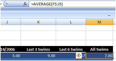
As you can see in the screenshot below, once you have added and deleted columns, this no longer works as a solution:

=AVERAGE(INDIRECT("B" & ROW() & ":J" & ROW()))
Summary
Sometimes Excel seems to work so hard to be helpful that it works against what you want, but there is almost always a way to get the result you need. Lucky for us in this case the INDIRECT() function is an easy solution!
P.S.
Don’t forget to check out our PDF to Excel Converter. It can save you a lot of precious time and improve your productivity.


