The Microsoft Excel VLOOKUP() function is one of the most useful but confused spreadsheet functions. It allows you to look up a value in a range based on a value of an ‘index column’.
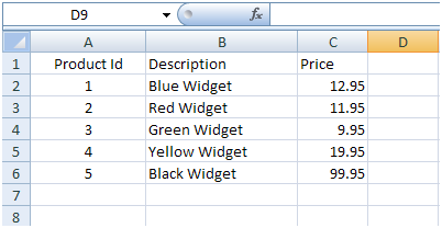
In the table below, you can see a standard product list:


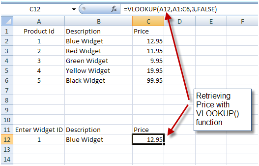
- The first parameter of the VLOOKUP() function is the value to look for. In our case it is the Product ID found in cell A12.
- The second parameter is the range where we want to look for the value. In our case, it is the range containing the products table: A1:C6.
- The third parameter is the column from which the value will be returned. In our case it is the third column in the range, which is column C (The price column).
- The fourth column indicates whether the VLOOKUP() function will look for an exact match or if it will settle for a close match. In our case we selected FALSE which says – Exact match.
If you are already familiar with VLOOKUP then you know how powerful a function it is. And if you have just heard about it now – congratulations, you have become a better Excel user.
The problem with VLOOKUP()
VLOOKUP is very useful, but it also has a lot of limitations. One of the most obvious limitations is that you can only look up a value based on one parameter. Another obvious problem is that you can only find rows that exactly match the parameter. You can’t define logical rules such as ‘bigger than’, ‘smaller than’ and so on.
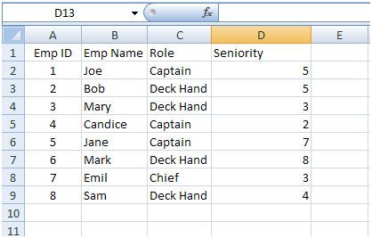
So, if we wanted to retrieve an employee from the following table. A deck hand that has 8 or more years of seniority, for example, we would not be able to use the VLOOKUP function.


- First we create an array, that has 1 column and as many rows as our lookup table. This array will hold the value 1 for each row in the lookup table that has the value ‘Deck Hand’ in the Role column and holds a number greater or equal in the ‘Seniority’ column.
This is done by this expression:(C1:C9="Deck Hand")*1*(D1:D9>=8)*1
When this expression is entered as a formula (you need to enter this formula with CTRL+SHIFT+ENTER because it is an array formula), it will return two arrays of 1s and 0s and multiply them. The result would be the array described above.
- In the second step, we use the MATCH() function to find the location (the index) of the cell that contains 1 within the array.
- We use the INDEX() function to retrieve the employee name from column B, based on the index of the row that we discovered above.
Summary
If you found it difficult to follow the above, the best approach to learning this technique is to give it a try in your own project. You will quickly see how powerful it is!
This formula template can be used to retrieve values based on any number of parameters and is a de-facto, multi-parameter VLOOKUP function.
P.S.
Don’t forget to check out our PDF To Excel Converter. It can save you a lot of precious time you now spend on retyping PDF data.


